
On this page0% through guide
Exploring One-Variable Data and Collecting Data
Good statistics begins with a defensible question, design, and description.
What you’ll learn
- Describe distributions using shape, center, spread, and unusual features.
- Distinguish random sampling from random assignment.
- Recognize bias and choose an appropriate data-collection design.
Before you begin
An observational unit is the person or object measured. A variable records a characteristic of that unit. Categorical values place units into groups; quantitative values describe numerical amounts for which arithmetic has a useful meaning.
Explain these starting ideas in your own words. Revisit them whenever a later step feels unclear.
Define the individuals, variable, and population
An individual is the object described by data, such as a student, household, or manufactured part. A variable records a characteristic. Categorical variables classify individuals, while quantitative variables measure numerical amounts for which arithmetic is meaningful. An identification number is not automatically quantitative just because it contains digits.
A population is the full group of interest; a sample is the observed subset. A parameter describes the population, while a statistic describes a sample. State the population and measurement method before calculating: the average for volunteers who complete an online survey may not estimate the intended population well.
Choose a display that fits the variable
Bar charts display category counts or proportions with distinct categories. Histograms group quantitative values into intervals, while dotplots and stemplots can preserve individual values in smaller datasets. A boxplot summarizes center and quartiles but can conceal clusters or gaps that a fuller display reveals.
Describe a quantitative distribution in context using shape, center, spread, and unusual features. When comparing groups, make direct comparisons rather than writing two disconnected descriptions. Include units and specify the measure of spread, such as IQR or standard deviation. A long right tail indicates right skew even if most observations lie toward the left.
Center and spread respond differently to extremes
The mean uses every value and is sensitive to extreme observations. The median is the middle ordered value and is resistant. Standard deviation describes typical distance from the mean through squared deviations; IQR is Q3 − Q1 and summarizes the middle half. Neither measure is the full range.
The 1.5-IQR rule flags potential outliers below Q1 − 1.5IQR or above Q3 + 1.5IQR. A flag is a prompt for investigation, not automatic permission to delete data. Adding a constant shifts center but not spread. Multiplying values by a constant scales spread by its absolute value.
Read figure values as text
Mean (14+x)/5: 6: 4; 6.416666666666667: 4.083333333333334; 6.833333333333333: 4.166666666666666; 7.25: 4.25; 7.666666666666667: 4.333333333333334; 8.083333333333334: 4.416666666666667; 8.5: 4.5; 8.916666666666666: 4.583333333333333; 9.333333333333334: 4.666666666666667; 9.75: 4.75; 10.166666666666668: 4.833333333333334; 10.583333333333332: 4.916666666666666; 11: 5; 11.416666666666668: 5.083333333333334; 11.833333333333332: 5.166666666666666; 12.25: 5.25; 12.666666666666668: 5.333333333333334; 13.083333333333332: 5.416666666666666; 13.5: 5.5; 13.916666666666668: 5.583333333333334; 14.333333333333334: 5.666666666666667; 14.75: 5.75; 15.166666666666666: 5.833333333333333; 15.583333333333334: 5.916666666666667; 16: 6; 16.416666666666664: 6.083333333333333; 16.833333333333336: 6.166666666666667; 17.25: 6.25; 17.666666666666664: 6.333333333333333; 18.083333333333336: 6.416666666666667; 18.5: 6.5; 18.916666666666664: 6.583333333333333; 19.333333333333336: 6.666666666666667; 19.75: 6.75; 20.166666666666664: 6.833333333333333; 20.583333333333336: 6.916666666666667; 21: 7; 21.416666666666664: 7.083333333333333; 21.833333333333336: 7.166666666666667; 22.25: 7.25; 22.666666666666668: 7.333333333333334; 23.083333333333332: 7.416666666666666; 23.5: 7.5; 23.916666666666668: 7.583333333333334; 24.333333333333332: 7.666666666666666; 24.75: 7.75; 25.166666666666668: 7.833333333333334; 25.583333333333332: 7.916666666666666; 26: 8 • Median: 6: 4; 6.416666666666667: 4; 6.833333333333333: 4; 7.25: 4; 7.666666666666667: 4; 8.083333333333334: 4; 8.5: 4; 8.916666666666666: 4; 9.333333333333334: 4; 9.75: 4; 10.166666666666668: 4; 10.583333333333332: 4; 11: 4; 11.416666666666668: 4; 11.833333333333332: 4; 12.25: 4; 12.666666666666668: 4; 13.083333333333332: 4; 13.5: 4; 13.916666666666668: 4; 14.333333333333334: 4; 14.75: 4; 15.166666666666666: 4; 15.583333333333334: 4; 16: 4; 16.416666666666664: 4; 16.833333333333336: 4; 17.25: 4; 17.666666666666664: 4; 18.083333333333336: 4; 18.5: 4; 18.916666666666664: 4; 19.333333333333336: 4; 19.75: 4; 20.166666666666664: 4; 20.583333333333336: 4; 21: 4; 21.416666666666664: 4; 21.833333333333336: 4; 22.25: 4; 22.666666666666668: 4; 23.083333333333332: 4; 23.5: 4; 23.916666666666668: 4; 24.333333333333332: 4; 24.75: 4; 25.166666666666668: 4; 25.583333333333332: 4; 26: 4
PAUSE & TRY IT
Which is usually more resistant to a single extreme high value, mean or median?
Reveal answer
The median, because it depends primarily on order rather than the magnitude of every value.
Normal models are assumptions about distributions
A normal distribution is symmetric and bell shaped, specified by a mean and standard deviation. Standardizing maps a value to its relative location in standard-deviation units. Probabilities correspond to areas under the density curve, not the curve’s height at one point.
Use a normal model only when it is appropriate or explicitly given. The empirical rule approximates 68%, 95%, and 99.7% within one, two, and three standard deviations. A percentile describes the proportion at or below a value under the stated convention; a z-score is not itself a probability.
Group A (min, Q1, median, Q3, max): 30, 42, 50, 58, 70 • Group B (min, Q1, median, Q3, max): 10, 30, 50, 70, 90
Random sampling supports population inference
A simple random sample gives each possible sample of the stated size an equal chance of selection. Stratified sampling divides the population into meaningful groups and samples within each; cluster sampling randomly selects groups and samples all or some individuals within them according to the design. Systematic sampling uses a random start and regular interval, with attention to possible periodic patterns.
Undercoverage leaves some population members inadequately represented. Nonresponse occurs when selected individuals do not provide data. Voluntary-response samples can overrepresent people motivated to participate. Response bias arises when wording, memory, social pressure, or measurement systematically distorts responses. Increasing sample size reduces random variability but does not automatically remove bias.
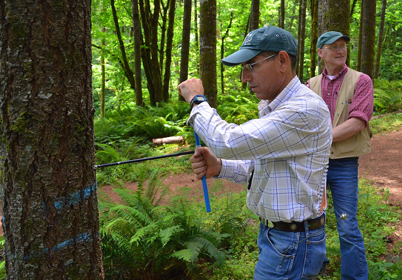
Field observations need a sampling frame, consistent measurements, and independent sampling units. Accessible locations alone can misrepresent the forest. This photograph illustrates fieldwork rather than supplying the numerical examples in this guide.
Photo: NRCS Oregon / USDA · Source · U.S. federal government public domain · Unmodified.PAUSE & TRY IT
What distinguishes bias from random sampling variability?
Reveal answer
Bias is a systematic tendency in a method; random variability is chance fluctuation among samples.
Random assignment supports causal comparison
An observational study records existing conditions without assigning treatments. An experiment imposes treatments. Random assignment helps balance lurking variables across groups, supporting a causal comparison when implementation is sound. Random sampling and random assignment serve different purposes; one does not replace the other.
Control, replication, and randomization strengthen experiments. Blocking groups similar experimental units before random assignment can reduce variability. A matched-pairs design compares naturally paired observations or two conditions on the same unit with appropriate order control. Blinding can reduce expectation effects, while a placebo can help separate treatment effects from the experience of receiving a treatment.
PAUSE & TRY IT
Why does blocking help?
Reveal answer
It groups similar units so comparisons within blocks can reduce variation unrelated to treatment.
Match the conclusion to the design
A well-randomized experiment may support causation for the studied units but not broad population generalization if the subjects are a narrow convenience sample. A representative observational sample may support an association in a population but not establish causation. Confounding occurs when effects of explanatory variables cannot be separated.
An ethical design requires informed participation and appropriate treatment of subjects. Missing data, dropouts, and noncompliance can undermine an otherwise good assignment procedure. Report limitations directly and avoid claiming that statistical sophistication repairs a fundamentally biased design.
Choose a representation that answers the question
Begin by identifying the observational units, the variable, and the population you want to understand. A histogram groups quantitative observations into intervals, so its shape depends partly on bin width. A boxplot emphasizes quartiles, median, spread, and potential outliers but hides clusters and gaps. Do not infer a detailed distribution shape from a boxplot alone.
Compare distributions using context, shape, center, variability, and unusual observations. “Group A is better” is not a statistical description. A stronger statement says which measured quantity has the higher typical value and which group varies more. For a strongly skewed distribution, the median and interquartile range often describe typical values more robustly than the mean and standard deviation.
PAUSE & TRY IT
Why does a larger convenience sample not necessarily remove bias?
Reveal answer
It reduces some random variability but does not repair systematic undercoverage or self-selection.
Separate random selection from random assignment
Random selection supports generalizing from a sample to its population. Random assignment supports a causal comparison by distributing potential confounding variables across treatment groups. These are different design decisions. A randomized experiment using volunteers can support a causal conclusion for the participants without establishing that its effect generalizes to all students.
In a blocked experiment, first create groups whose members are similar on a variable expected to affect the response, then randomly assign treatments within each block. Blocking reduces unwanted variability; it does not replace random assignment. A matched-pairs design compares related observations, such as two measurements on each participant, so the analysis should preserve those pairs.
Random sampling produces one sample and a statistic. Repeating the process gives a sampling distribution that describes variability in that statistic.
PAUSE & TRY IT
Why should a pretest–posttest study preserve each person’s pair?
Reveal answer
The within-person difference removes some person-to-person variability and represents the intended response.
Explain why a sampling method can be biased
Sampling variability is the chance fluctuation among statistics from repeated random samples. Bias is a tendency for a method to systematically miss the population value in a particular direction. Increasing a biased sample from 100 to 10,000 does not automatically correct the selection process. A large voluntary-response poll can still overrepresent people with especially strong opinions.
Identify the mechanism and likely direction when possible. If a survey about commuting time reaches only people arriving before 8 a.m., it may omit a different commuting population. However, do not invent a direction without information connecting the omitted people to the response. State what is missing and why representativeness is uncertain.
Start with the observational unit and variable
Before calculating, identify one observational unit and what is measured on it. A numerical label such as a postal code is categorical because arithmetic on its digits does not measure a quantitative attribute. A count and a measurement can both be quantitative, but their possible values differ. This choice determines sensible displays and summaries.
Describe a quantitative distribution in context using shape, center, spread, and unusual features. A mean is pulled toward extreme observations; a median depends on order. Standard deviation measures typical distance from the mean in the variable’s units, while the IQR describes the middle half. A right-skewed distribution often has mean greater than median, but do not infer an exact mean from an unlabeled sketch.
Compare distributions explicitly: name which has the larger center or spread, rather than writing two disconnected descriptions. Check axes and sample sizes. A histogram’s bar height may represent frequency, relative frequency, or density; unequal bin widths require particular care. A boxplot conceals some shape information, so it cannot establish every feature visible in raw data.
Distinguish a sample design from an experiment
Random sampling supports generalization to the population represented by the sampling frame, subject to response and coverage limitations. Random assignment balances potential confounders across treatment groups in expectation and supports causal comparison. These are different random processes. An experiment using volunteers can support a causal claim for the studied setting without making the volunteers a random sample of everyone.
In a stratified sample, sample from each relevant subgroup. In a cluster sample, randomly select groups and observe units within those groups according to the design. The names are not interchangeable: stratification aims to represent subgroups, while clustering often improves practicality. A convenience sample with many responses remains vulnerable to selection bias.
Undercoverage, nonresponse, and response bias affect different parts of data collection. An online survey can miss people without access; selected people may not respond; wording can influence answers. Increasing sample size reduces random sampling variability but does not automatically repair these systematic problems.
PAUSE & TRY IT
A voluntary survey has 100,000 responses. Does its size eliminate selection bias?
Reveal answer
No. A large sample can have little random variability while systematically overrepresenting people who choose to respond.
Design a comparison that can answer the question
An experiment needs clear treatments, an outcome, replication, and an assignment procedure. A control group provides a comparison; a placebo can help isolate effects of receiving treatment. Blinding reduces behavior or assessment changes caused by knowing treatment assignment. Explain who is blinded and why it matters.
Blocking groups units using a relevant pre-treatment characteristic, then randomizes treatments within blocks. A matched-pairs design can use the same person under two conditions or carefully matched units. Pairing changes the analysis because differences within pairs, rather than all individual observations treated as independent, become central.
Confounding occurs when effects cannot be separated. If every treated plant is in one greenhouse and every control plant in another, greenhouse and treatment are confounded. Many leaves measured on one plant do not create many independently treated plants. Identify the actual experimental unit before counting replication.
FROM IDEA TO APPLICATION
Worked examples
Transform a distribution
Commute times have mean 24 minutes and standard deviation 6 minutes. A new variable records time in seconds plus a fixed 30-second setup delay. Find its mean and standard deviation.
Reveal worked solution
- The transformation is Y = 60X + 30.
- Mean becomes 60(24) + 30 = 1,470 seconds.
- Standard deviation becomes |60|(6) = 360 seconds; adding 30 does not change spread.
Mean 1,470 seconds; standard deviation 360 seconds.
What conclusion is justified?
Volunteers are randomly assigned to two study methods. One group scores higher. Can the result establish causation and generalize to every student?
Reveal worked solution
- Random assignment supports a causal comparison within the experiment if other design conditions are met.
- Volunteering is not random sampling from all students.
- Broad generalization requires caution about who volunteered and how the study was run.
The design can support a treatment-effect claim for the experimental context, but it does not by itself justify generalizing to every student.
A convincing design conclusion
A researcher randomly assigns 80 volunteer students to two study methods. The new method yields higher scores. What can random assignment establish, and what remains limited?
Reveal worked solution
- Random assignment makes treatment groups comparable in expectation, supporting a causal interpretation if the difference is statistically convincing.
- The students volunteered; they were not randomly selected from all students.
- Separate the causal conclusion for this experiment from the population-generalization limitation.
The design can support evidence that the method caused a score difference for these participants. Broad generalization requires additional justification.
Repair a confounded plant study
All 30 fertilized plants are grown under one lamp; all 30 controls under a second lamp.
Reveal worked solution
- Lamp and fertilizer treatment vary together.
- Differences could reflect lighting rather than fertilizer.
- Randomize fertilizer treatments within each suitable lighting block, with independent plants assigned to each treatment.
More leaves measured on the same plants cannot remove the lamp–treatment confounding.
MAKE THE DISTINCTION
Common mistakes, clearer reasoning
The trapA very large convenience sample removes selection bias.
The better explanationLarger samples reduce random sampling variability, not systematic selection problems.
The trapRandom sampling and random assignment are interchangeable.
The better explanationSampling supports representation; assignment supports causal treatment comparison.
RETRIEVE BEFORE YOU REVEAL
Practice checkpoints
Revisit the quick checks from this guide without looking back. Explain why, then reveal the answer.
1. Which is usually more resistant to a single extreme high value, mean or median?
Reveal answer
The median, because it depends primarily on order rather than the magnitude of every value.
2. Why does blocking help?
Reveal answer
It groups similar units so comparisons within blocks can reduce variation unrelated to treatment.
3. What distinguishes bias from random sampling variability?
Reveal answer
Bias is a systematic tendency in a method; random variability is chance fluctuation among samples.
4. Why does a larger convenience sample not necessarily remove bias?
Reveal answer
It reduces some random variability but does not repair systematic undercoverage or self-selection.
5. Why should a pretest–posttest study preserve each person’s pair?
Reveal answer
The within-person difference removes some person-to-person variability and represents the intended response.
6. A voluntary survey has 100,000 responses. Does its size eliminate selection bias?
Reveal answer
No. A large sample can have little random variability while systematically overrepresenting people who choose to respond.
Key language
- Parameter
- A numerical characteristic of a population.
- Statistic
- A numerical characteristic calculated from a sample.
- Confounding
- An inability to separate the effects of explanatory variables.
- Random assignment
- Use of chance to allocate experimental units to treatments.
Inference procedures rely on the sampling and assignment assumptions established here.